Changes in Novartis’ News Coverage
3 min
This notebook allows you to get up and running quickly with the Sturdy Statistics API. We will create a series of visualization to explore past two years of Earnings Calls from Google, Microsoft, Amazon, NVIDA, and META. Earnings Calls are a quarterly event during which a public company will discuss the results of the past quarter and take questions from its investors. These calls offer a unique candid glimpse into both the company’s outlooks as well as that of the tech industry as a whole.
We will be using an index from our pretrained gallery for this analysis. You can sign up on our website to generate your free, no payment info required, API key to run this notebook yourself and to upload your own data for analysis.
pip install sturdy-stats-sdk pandas numpy plotly
# pip install sturdy-stats-sdk pandas numpy plotly duckdb
from IPython.display import display, Markdown, Latex
import pandas as pd
import numpy as np
import plotly.express as px
from sturdystats import Index, Job

from pprint import pprint

index_id = "index_c6394fde5e0a46d1a40fb6ddd549072e"
index = Index(id=index_id)## Basic Utilities
from plotly import io as pio
px.defaults.template = "simple_white" # Change the template
px.defaults.color_discrete_sequence = px.colors.qualitative.Dark24 # Change color sequence
pio.templates["no_margins"] = pio.templates["simple_white"].update({
"layout": {
"margin": {"l": 0, "r": 0, "t": 30, "b": 0, "pad": 0}
}
})
# Set it as default template
pio.templates.default = "no_margins"
def procFig(fig, **kwargs):
fig.update_layout(plot_bgcolor= "rgba(0, 0, 0, 0)", paper_bgcolor= "rgba(0, 0, 0, 0)",
margin=dict(l=0,r=0,b=0,t=30,pad=0),
**kwargs
)
fig.layout.xaxis.fixedrange = True
fig.layout.yaxis.fixedrange = True
return fig
def displayText(df, highlight):
def processText(row):
t = "\n".join([ f'1. {r["short_title"]}: {int(r["prevalence"]*100)}%' for r in row["paragraph_topics"][:5] ])
x = row["text"].replace("*", "").replace("$", "")
res = []
for word in x.split(" "):
for term in highlight:
if term.lower() in word.lower() and "**" not in word:
word = "**"+word+"**"
res.append(word)
return f"<em>\n\n#### Result {row.name+1}/{df.index.max()+1}\n\n##### {row['ticker']} {row['pub_quarter']}\n\n"+ t +"\n\n" + " ".join(res) + "</em>"
res = df.apply(processText, axis=1).tolist()
display(Markdown(f"\n\n...\n\n".join(res)))The core building block in the Sturdy Statistics NLP toolkit is the Index. Each Index is a set of documents and metadata that has been structured or “indexed” by our hierarchical bayesian probability mixture model. Below we are connecting to an Index that has already been trained by our earnings transcripts integration.
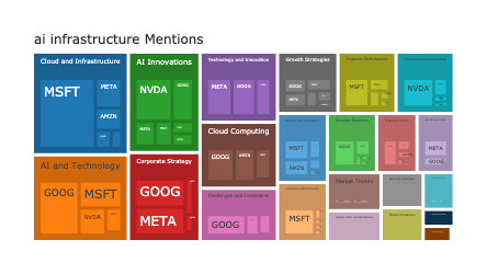
index = Index(id="index_c6394fde5e0a46d1a40fb6ddd549072e") Found an existing index with id="index_c6394fde5e0a46d1a40fb6ddd549072e".The first API we will explore is the Topic Search API. This API provides a direct interface to the high level themes that our index extracts. You can call with no arguments to get a list of topics ordered by how often they occur in the dataset (prevalence). The resulting data is a structured rollup of all the data in the corpus. It aggregates the topic annotations across each word, paragraph, and document and generates high level semantic statistics.
Mentions refers to the number of paragraphs in which the topic occurs. Prevalence refers to the total percentage of all data that a topic comprises.
topic_df = index.topicSearch()
topic_df.head()[["topic_id", "short_title", "topic_group_short_title", "mentions", "prevalence"]]| topic_id | short_title | topic_group_short_title | mentions | prevalence | |
|---|---|---|---|---|---|
| 0 | 159 | Accelerated Computing Systems | Technological Developments | 359.0 | 0.042775 |
| 1 | 139 | Consumer Behavior Insights | Growth Strategies | 585.0 | 0.033129 |
| 2 | 108 | Cloud Performance Metrics | Investment and Financials | 157.0 | 0.026985 |
| 3 | 115 | Zuckerberg on Business Strategies | Corporate Strategy | 420.0 | 0.026971 |
| 4 | 127 | Comprehensive Security Solutions | Investment and Financials | 146.0 | 0.023265 |
We can quickly visualize this topic dataframe in a pie chart using plotly. The size of each slice of the pie chart represents how prominent a topic is.
This visual is very fast and useful, but quickly becomes overwhelming if we attempt to display too many topics
import plotly.express as px

topic_df["title"] = "Tech <br> Earnings Calls"
fig = px.sunburst(
    topic_df.head(100),
    path=["title", "short_title"],
    values="prevalence",
    hover_data=["topic_id", "mentions"],
    height=500
)
fig.show()We can better visualize our thematic data by leveraging Sturdy Statistic’s hierarchical schema. We can display this hierarchy using a Sunburst visualization. The inner circle of the sunburst is the title of the plot. And the leaf nodes are the same topics topics that we displayed in the pie chart above. The middle layer is the topic_group, which Sturdy Statistics automatically extracts in conjunction with the granular topics. The size of each slice is porportional to how often it shows up in the dataset.
import plotly.express as px

topic_df["title"] = "Tech <br> Earnings Calls"
fig = px.sunburst(
    topic_df,
    path=["title", "topic_group_short_title", "short_title"],
    values="prevalence",
    hover_data=["topic_id", "mentions"],
    height=500
)
fig.show()The Topic Search API (along with our other semantic APIs) produce high level insights. In order to both dive deeper into and verify these insights, we provide a mechanism to retrieve the underlying data with our query API. This API shares a unified filtering engine with our higher level semantic APIs. Any semantic rollup or insight aggregation can be instantly “unrolled”.
Let’s take the topic AI Model Scaling. We can uncover the topic metadata below and see that it was mentioned 81 times in the corpus.
TOPIC_ID = 53
row = topic_df.loc[topic_df.topic_id == TOPIC_ID]
row[["topic_id", "short_title", "mentions"]]| topic_id | short_title | mentions | |
|---|---|---|---|
| 81 | 53 | AI Model Scaling | 81.0 |
We can call the Query API, passing in our topic_id. We can see that we have 81 mentions returned, lining up exactly with our aggregate APIs.
df = index.query(topic_id=TOPIC_ID, max_excerpts_per_doc=200, limit=200) ## 200 is the single request limit
df.iloc[[0,-1]]| doc_id | text | ticker | quarter | pub_quarter | year | published | title | author | paragraph_id | metadata | predictions | doc_topics | paragraph_topics | search_score | topic_search_score | exact_match_search_score | |
|---|---|---|---|---|---|---|---|---|---|---|---|---|---|---|---|---|---|
| 0 | 8f55c1161342d07cc3a9a2be55d59dad | Jensen Huang: No. No. I'm gonna just wanna tha... | NVDA | 2025Q4 | 2025Q1 | 2025 | 2025-02-26 | NVDA 2025Q4 | NVDA | 55 | {'ticker': 'NVDA', 'quarter': '2025Q4', 'pub_q... | {} | [{'short_title': 'Accelerated Computing System... | [{'short_title': 'AI Model Scaling', 'topic_gr... | 10.079368 | 0.0 | 2.0 |
| 80 | 12b7f45254d6b5326307df2bad8def95 | Ross Sandler: Great. Just two quick ones, Mark... | META | 2024Q3 | 2024Q4 | 2024 | 2024-10-30 | META 2024Q3 | META | 36 | {'ticker': 'META', 'quarter': '2024Q3', 'pub_q... | {} | [{'short_title': 'Zuckerberg on Business Strat... | [{'short_title': 'Business Growth Strategies',... | 10.079368 | 0.0 | 2.0 |
Below we display the first and last result of our query results. Unlike neural embeddings, the sparse structure that our Index learns enables us to set hard semantic thresholds.
Because our model annotates every single word in a document, we can extract the specific terms that lead to the high topic score in each excerpt. We leverage
You will notice that accompanying each excerpt is a set of tags. These are the same tags that are returned in our Topic Search API. Here each tag corresponds to the percentage of the paragraph that it comprises.
def display_text(df, highlight):
    import re
    try:
        from IPython.display import display, Markdown
        show = lambda x: display(Markdown(x))
    except ImportError:
        show = print
    def fmt(r):
        t = "\n".join(f"1. {d['short_title']}: {int(d['prevalence']*100)}%" for d in r["paragraph_topics"][:5])
        txt = re.sub(r"[*$]", "", r["text"])
        h = lambda m: f"**{m.group()}**" \
            if any((len(w) < 4 and m.group().lower() == w.lower()) \
            or (len(w) >= 4 and w.lower() in m.group().lower()) for w in highlight) else m.group()
        body = re.sub(r"\b\w+\b", h, txt)
        return f"<em>\n\n#### Result {r.name+1}/{df.index.max()+1}\n\n##### {r['ticker']} {r['pub_quarter']}\n\n{t}\n\n{body}</em>"
    show("\n\n...\n\n".join(df.apply(fmt, axis=1)))
topicWords = index.topicWords()
words_to_highlight = topicWords.loc[topicWords.topic_id == TOPIC_ID].topic_words.explode().tolist()
display_text(df.iloc[[0, -1]], highlight=words_to_highlight)
assert len(df) == row.iloc[0].mentions
Jensen Huang: No. No. I’m gonna just wanna thank you. Up to, Jensen? And, like, the medium, a couple things. I just wanna thank you. Thank you, Colette. Demand for Blackwell is extraordinary. AI is evolving beyond perception. And generative AI into reasoning. With reasoning AI, we’re observing another scaling law. Inference time or test time scaling. The more computation the more the model thinks the smarter the answer. Models like OpenAI’s Grok 3, DeepSeq R1, are reasoning models that apply inference time scale. Reasoning models can consume a hundred times more compute. Future reasoning models can consume much more compute. DeepSeq R1 has ignited global enthusiasm. It’s an excellent innovation. But even more importantly, it has open-sourced a world-class reasoning AI model. Nearly every AI developer is applying R1. Or chain of thought and reinforcement learning techniques like R1. To scale their model’s performance. We now have three scaling laws, as I mentioned earlier. Driving the demand for AI computing. The traditional scaling laws of AI remain intact. Foundation models are being enhanced with multimodality. And pretraining is still growing. But it’s no longer enough. We have two additional scaling dimensions. Post-training scaling, where reinforcement learning fine-tuning, model distillation, require orders of magnitude more compute than pretraining alone.
…
Ross Sandler: Great. Just two quick ones, Mark. You said something along the lines of the more standardized Llama becomes, the more improvements will flow back to the core Meta business. And I guess, could you dig in a little bit more on that? So the series of Llama models are being used by lots of developers building different things in AI. I guess, how are you using that vantage point to incubate new ideas inside Meta? And then second question is, you mentioned on one of the podcasts after the Meta Connect that assuming scaling laws hold up, we may need hundreds of billions of compute CapEx to kind of reach our goals around Gen AI. So I guess how quickly could you conceivably stand up that much infrastructure given some of the constraints around energy or custom ASICs or other factors? Is there any more color on the speed by which we could get that amount of compute online at Meta? Thank you.
Our model granularly annotates every word, sentence, paragraph and document with topic information. The structured nature of our semantic data allows us to store this data in a structured tabular format alongside any relevant metadata. This means we can perform complex semantic analyses directly in SQL.
AI Model Scaling over TimeThe SQL statement below is a standard group by. The only new content is the line: (sparse_list_extract({TOPIC_ID+1}, c_mean_avg_inds, c_mean_avg_vals) > 2.00)::INT. Sturdy Statistics stores thematic content arrays in a sparse format of a list of indices and a list of values. This format provides significant storage and performance optimizations. We use a defined set of sparse functions to work with this data.
Below we give it the fields c_mean_avg_inds and c_mean_avg_vals. The original c_mean_avg array is a count of the number of words in each paragraph that have been assigned to a topic. The mean_avg denotes that this value has been accumulated over several hundred MCMC samples. This sampling has numerous benefits and is also why our counts are not integers (a very common question we receive).
TOPIC_ID = 53
df = index.queryMeta(f"""
SELECT
    pub_quarter,
    sum(
        (sparse_list_extract({TOPIC_ID+1}, c_mean_avg_inds, c_mean_avg_vals) > 2.00)::INT
    ) as mentions
FROM paragraph
GROUP BY pub_quarter
ORDER BY pub_quarter
""")


fig = px.bar(
    df, x="pub_quarter", y="mentions",
    title=f"Mentions of 'AI Model Scaling'",
   # line_shape="hvh",
)
fig.update_layout(title_x=.5).show()Because this semantic data is stored directly in a SQL table, we can enrich our semantic analysis with metadata. Below, we are able to break how much each company is dicussing the topic AI Model Scaling and when they are talking about it.
TOPIC_ID = 53
df = index.queryMeta(f"""
SELECT
    pub_quarter,
    ticker,
    sum(
        (sparse_list_extract({TOPIC_ID+1}, c_mean_avg_inds, c_mean_avg_vals) > 2.00)::INT
    ) as mentions
FROM paragraph
GROUP BY pub_quarter, ticker
ORDER BY pub_quarter
""")


fig = px.bar(
    df, x="pub_quarter", y="mentions", color="ticker",
    title=f"Mentions of 'AI Model Scaling'",
)
fig.update_layout(title_x=.5).show()In addition to storing the thematic content directly in the SQL tables, we integrate our semantic search engine within SQL. Below we pass the semantic search query infrastructure as a filter for our analysis.
TOPIC_ID = 53
df = index.queryMeta(f"""
SELECT
    pub_quarter,
    ticker,
    sum(
        (sparse_list_extract({TOPIC_ID+1}, c_mean_avg_inds, c_mean_avg_vals) > 2.00)::INT
    ) as mentions
FROM paragraph
GROUP BY pub_quarter, ticker
ORDER BY pub_quarter
""",
search_query="infrastructure")


fig = px.bar(
    df, x="pub_quarter", y="mentions", color="ticker",
    title=f"Mentions of 'AI Model Scaling'",
)
fig.update_layout(title_x=.5).show()As always, any high level insights can be tied back to the underlying data that comprises it. Below, we pull up all examples of AI Model Scaling that focus on the search term Infrastructure during Meta’s 2025Q1 earning’s call. We assert that there are 4 examples (the value our bar chart provides) returned and we display the first and last ranked example.
Note that the last example does not explicitly mention Infrastructure but instead matches on terms such as CapEx and data centers.
df = index.query(topic_id=TOPIC_ID, search_query='infrastructure',
                 filters="ticker='META' AND pub_quarter='2025Q1'")
words_to_highlight = topicWords.loc[topicWords.topic_id == TOPIC_ID].topic_words.explode().tolist()
display_text(df.iloc[[0, -1]], words_to_highlight)
assert len(df) == 4
Mark Zuckerberg: I can start on the DeepSeek question. I think there’s a number of novel things that they did that I think we’re still digesting. And there are a number of things that they have advances that we will hope to implement in our systems. And that’s part of the nature of how this works, whether it’s a Chinese competitor or not. I kind of expect that every new company that has an advance – that has a launch is going to have some new advances that the rest of the field learns from. And that’s sort of how the technology industry goes. I don’t know – it’s probably too early to really have a strong opinion on what this means for the trajectory around infrastructure and CapEx and things like that. There are a bunch of trends that are happening here all at once. There’s already sort of a debate around how much of the compute infrastructure that we’re using is going to go towards pretraining versus as you get more of these reasoning time models or reasoning models where you get more of the intelligence by putting more of the compute into inference, whether just will mix shift how we use our compute infrastructure towards that. That was already something that I think a lot of the other labs and ourselves were starting to think more about and already seemed pretty likely even before this, that – like of all the compute that we’re using, that the largest pieces aren’t necessarily going to go towards pre-training.
…
Susan Li: I’m happy to add a little more color about our 2025 CapEx plans to your second question. So we certainly expect that 2025 CapEx is going to grow across all three of those components you described. Servers will be the biggest growth driver that remains the largest portion of our overall CapEx budget. We expect both growth in AI capacity as we support our gen AI efforts and continue to invest meaningfully in core AI, but we are also expecting growth in non-AI capacity as we invest in the core business, including to support a higher base of engagement and to refresh our existing servers. On the data center side, we’re anticipating higher data center spend in 2025 to be driven by build-outs of our large training clusters and our higher power density data centers that are entering the core construction phase. We’re expecting to use that capacity primarily for core AI and non-AI use cases. On the networking side, we expect networking spend to grow in ’25 as we build higher-capacity networks to accommodate the growth in non-AI and core AI-related traffic along with our large Gen AI training clusters. We’re also investing in fiber to handle future cross-region training traffic. And then in terms of the breakdown for core versus Gen AI use cases, we’re expecting total infrastructure spend within each of Gen AI, non-AI and core AI to increase in ’25 with the majority of our CapEx directed to our core business with some caveat that, that is – that’s not easy to measure perfectly as the data centers we’re building can support AI or non-AI workloads and the GPU-based servers, we procure for gen AI can be repurposed for core AI use cases and so on and so forth.
At any point, we can also zoom back out into the high level topic view. Instead of focusing in on the AI Model Scaling topic, we can instead zoom out and see everything Meta discussed about infrastructure during 2025Q1’s earning call.
topic_df = index.topicSearch("infrastructure", filters="ticker='META' and pub_quarter='2025Q1'")
topic_df["title"] = "Meta 2025Q1 Discussions"
fig = px.sunburst(
    topic_df,
    path=["title", "short_title"],
    values="prevalence",
    hover_data=["topic_id", "mentions"]
)
fig.update_layout(height=500).show()In addition to power our semantic APIs, Sturdy Statistics’ probability model also powers our statistical search engine. When you submit a search query, your index model maps your query to its thematic contents. Because our models return structured Bayesian likelihoods, we are able use a statistically meaningful scoring metric called hellinger distance to score each search candidate. Unlike cosine distance whose values are not well defined and can be used only to rank, the hellinger distance score defines the percentage of a document that ties directly to your theme.
This well defined score enables not only search ranking, but semantic search filter as well with the ability to define a hand-selected hard cutoff
We are using two new capabilities in the Query API: filtering and search. Our Query API supports arbitrary sql conditions in the filter. We leverage DuckDB under the hood and support all of DuckDB’s sql querying syntax.
In addition to accepting a search term, our Query API accepts a semantic_search_cutoff and a semantic_search_weight. The semantic_search_cutoff is a value between 0-1. The value corresponds to the percentage of the paragraph that focuses on the search term. Our value of .1 below means that at least 10% of the paragraph must focus on our search term. This enables flexible semantic filtering capabilities while providing sensible defaults out of the box.
The semantic_search_weight dictates the weight placed on our thematic search score vs our TF-IDF weighted exact match score. Each use case is different and our API provides the flexibility to tune you indices according to your use-case while providing sensible defaults out of the box.
In the examples below, you’ll notice that our index surfaced paragraphs that matched not only on FX, but also on foreign exchange, pressures, and slowdown.
def display_text(df, highlight):
    import re
    try:
        from IPython.display import display, Markdown
        show = lambda x: display(Markdown(x))
    except ImportError:
        show = print
    def fmt(r):
        t = "\n".join(f"1. {d['short_title']}: {int(d['prevalence']*100)}%" for d in r["paragraph_topics"][:5])
        txt = re.sub(r"[*$]", "", r["text"])
        h = lambda m: f"**{m.group()}**" \
            if any((len(w) < 4 and m.group().lower() == w.lower()) \
            or (len(w) >= 4 and w.lower() in m.group().lower()) for w in highlight) else m.group()
        body = re.sub(r"\b\w+\b", h, txt)
        return f"<em>\n\n#### Result {r.name+1}/{df.index.max()+1}\n\n##### {r['ticker']} {r['pub_quarter']}\n\n{t}\n\n{body}</em>"
    show("\n\n...\n\n".join(df.apply(fmt, axis=1)))
SEARCH_QUERY = "fx"
FILTER = "ticker='GOOG'"
df = index.query(SEARCH_QUERY, filters=FILTER,
semantic_search_cutoff=.1, semantic_search_weight=.3,
max_excerpts_per_doc=20, limit=200)
topics = index.topicSearch(SEARCH_QUERY).iloc[:10]
words_to_highlight = topicWords.loc[topicWords.topic_id.apply(lambda x: x in topics.topic_id)].topic_words.explode()
display_text(df.iloc[[0, -1]], highlight=words_to_highlight) #highlight=["fx", "foreign", "exchange", "stabilization", "pressures", "slowdown", "pullback"])
Justin Post: Just digging into Search kind of low single-digit growth ex FX. Can you talk about the pressures there, volume versus pricing or CPCs? What’s really driving the slowdown? It’s kind of almost back to ‘09 recession levels. Just think about that. And then any signs that we’re near a bottom? Any stabilization in growth rates you can talk about or how your outlook is for’23 on that?
…
Google Services revenue of 62 billion were up 1% year-on-year, including the effect of a modest foreign exchange headwind. In Google Advertising, Search and Other, revenues grew 2% year-over-year, reflecting an increase in the travel and retail verticals, offset partially by a decline in finance as well as in media and entertainment. In YouTube Ads, we saw signs of stabilization and performance, while in network, there was an incremental pullback in advertiser spend. Google Other revenues were up 9% year-over-year led by strong growth in YouTube subscriptions revenues.
The exact match search only hits on a single result. We are missing 20/27 of the matching exchanges because of the restrictiveness of exact matching rules.
## Setting semantic search weight to 0 forces an exact match only search.
df = index.query(SEARCH_QUERY, filters=FILTER, semantic_search_cutoff=.1, semantic_search_weight=0, max_excerpts_per_doc=40, limit=200)
display_text(df.iloc[[0, -1]], highlight=["fx"])
I’ll highlight 2 other factors that affected our Ads business in Q4. Ruth will provide more detail. In Search and Other, revenues grew moderately year-over-year, excluding the impact of FX, reflecting an increase in retail and travel, offset partially by a decline in finance. At the same time, we saw further pullback in spend by some advertisers in Search in Q4 versus Q3. In YouTube and Network, the year-over-year revenue declines were due to a broadening of pullbacks in advertiser spend in the fourth quarter.
…
Anat Ashkenazi: And on the question regarding my comment on lapping the strength in financial services, this is primarily related to the structural changes with regards to insurance, it is more specifically within financial services, it was the insurance segment and we saw that continue, but it was a one-time kind of a step up and then we saw it throughout the year. I am not going to give any specific numbers as to what we expect to see in 2025, but I am pleased with the fact that we are seeing and continue to see strength across really all verticals including retail and exiting the year in a position of strength. If anything, I would highlight as you think about the year, the comments I have made about the impact of FX, as well as the fact that we have one less day of revenue in Q1.
In our FX search query, the data very useful, but that’s a lot to read and digest. Let’s try to summarize that data into a high level overview. Because our Topic Search API supports the exact same parameters as our Query API, we can instantly switch between high level insights and granular data.
df = index.topicSearch(SEARCH_QUERY, FILTER, semantic_search_cutoff=.1)
df["search_query"] = SEARCH_QUERY
fig = px.sunburst(df, path=["search_query", "short_title"], values="prevalence", hover_data=["topic_id"],)
procFig(fig, height=500).show()from sturdystats import Index
index = Index("Custom Analysis")
index.upload(df.to_dict("records"))
index.commit()
index.train()
# Ready to Explore
index.topicSearch()